Utilizing cOmicsArt for Iterative Data Analysis: From Data Input to Comprehensive Insights and Reproducibility
This showcase demonstrates how to use cOmicsArt to analyze and visualize data based on a specific dataset. As background information, the dataset used in this showcase comes from a study that investigates how a high-salt diet (HSD) impacts immune defense against kidney infections, utilizing transcriptomics data to explore these effects. The study finds that an HSD worsens pyelonephritis in mice by impairing neutrophil antibacterial function. This is due to urea accumulation and disrupted circadian glucocorticoid rhythms, which impair neutrophil function. For further information and additional data, please see the original publication by Jobin et al.[\^0]. The showcase is divided into sections: ‘The Data – Retrieval and preparation, Upload and Pre-processing’, ‘Investigating global patterns - Sample Correlation and PCA’, ‘Statistical Analysis’, ‘Intermediate Summary’, ‘Final Documentation’ and ‘Final Summary’. Each section provides insights from the analysis itself as well as how to obtain them using cOmicsArt. [\^0]: Jobin, K. et al. A high-salt diet compromises antibacterial neutrophil responses through hormonal perturbation. Sci Transl Med 12, (2020).
The Data - Retrieval and Preparation, Upload and Pre-processing
The raw count data and sample information were retrieved from the European Nucleotide Archive while the row annotation was created to fulfill cOmicsArt’s requirements. After uploading the data to the cOmicsArt web application, we requested additional gene annotations and performed pre-processing using the DESeq option, successfully generating homogeneous distributions across samples, as indicated by diagnostic plots.
Retrieval and Preparation:
The raw data (fastq files) and the sample information can be retrieved from the European Nucleotide Archive under the project PRJEB28204 (https://www.ebi.ac.uk/ena/browser/view/PRJEB28204). The data was aligned to the mm10 reference genome with the STAR Aligner.
Having the data in a count matrix format, we adjusted the corresponding sample and created the row annotation tables. The sample annotation table contains information about the samples, whereby we kept the information on the treatment, organism, cell type, and individual sample ID. We ensured that all samples listed in the column names of the count matrix also appear in the row names of the sample annotations. The required row annotation table containing information about the genes was not given but created. Here, we initially only had the gene Ensembl IDs taken from the count matrix. We ensured that all entities listed in the row names of the count matrix also appear in the row names of the row annotation. As a single column is minimally required for the row annotation, we added a column named ‘Ensembl_ID’, exactly coping the row names. Note, that there is extensive help with additional details for formatting data correctly within the documentation.
Within this showcase, we will come back to this step as we gain information throughout which we can add to our annotation table. All information provided in this step can be utilized during the analysis to filter and group the data or perform statistical tests on it.
Upload:
Upon creation of the sample and row annotation table, we can upload the data to the cOmicsArt web app. We select the omic type as transcriptomics and then provide the data matrix, the sample annotation, and finally the row annotation. A quick inspection of the data upon clicking the ‘inspect data’ button shows that the data was prepped correctly and we can proceed with the analysis. To do so, we click on ‘Upload new data’ and the data is loaded into the app.
As a first step, we add some more information to our entities. Specifically, we request cOmicsArt to add gene annotation on the basis of Mouse genes (GRCm39), which adds the gene names as well as the biotype of the genes to our entity annotation. Since we have named our initial column of the row annotation ‘Ensembl_ID’, cOmicsArt can automatically detect the correct column to use as the basis to add the additional info within the provided table. The automatic detection needs to be confirmed by the user. Note, that you need to have either Ensembl IDs, Entrez IDs, or gene names for the addition of information to work. Upon clicking the ‘Add Gene Annotation’ button, the data is added, before returning to the Data Upload tab to proceed.
For now, no selection of the data is done, such that all data is considered during the analysis, making us ready to ‘Start the Journey’ by clicking on the respective button.
Pre-processing:
For pre-processing, we select the DESeq option. Upon selection, we specify ‘Treatment’ as the main factor for the model. For more details about the DESeq2 pipeline used in the background, check out the DESeq2 vignette. The pre-processing involves filtering lowly expressed genes before applying the DESeq2 pipeline.

After clicking ‘Get Pre-Processing’, the data is processed and we can assess the diagnostic plots of the sample distribution (Fig. D1). We color the sample distribution diagnostic plots with respect to their treatment (side panel below the horizontal line, hence only performing re-coloring but no re-pre-processing). After preprocessing, we can see that the distribution across samples is similar and does not depend on the underlying treatment. We can conclude that the chosen pre-processing was successful in generating homogeneous distributions across samples.
Investigating global patterns - Sample Correlation and PCA
This section explores the correlation pattern among samples to determine if samples with similar treatments are more alike, utilizing sample correlation and principle component analysis.
Sample Correlation:
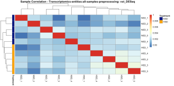
We first investigate whether global patterns within the data fit our expectations: samples with similar treatment are more similar to each other. Therefore, we assess their correlation pattern using the Pearson correlation coefficient within the sample correlation tab. Upon clicking ‘Get Sample Correlation’ we can observe that the correlation across all our samples is very high. Upon selecting ‘treatment’ as the annotation variable we can observe rather minor differences between the treatment groups (Fig. D2). This could indicate that the treatment does not have a strong effect on the global gene expression patterns. The expected effect is potentially only visible in a subset of the samples. Also, sample correlation incorporating all data might not be the best way to assess the effect of the treatment on such high-dimensional data. Hence, we further assess the PCA, to identify which linear combinations of features (here genes) explain the most variance within the data.
PCA:
Switching to the PCA-panel and performing a PCA colored after Treatment, we can observe that samples treated by HSD are less spread in the PC1 vs PC2 plot than the NSD samples (Fig. D3 A). Additionally, the samples have a separation tendency, although no clear separation is visible. We can also see that along PC1 (hence ‘from left to right’) two samples stand out on the left. Leveraging the tooltip (and changing ‘Select the anno to be shown at the tooltip’ to ‘individual_ID’) we can identify the samples NSD_1 and NSD_2 as distinct from the other samples along PC1.
Notable is the rather low numbers of observed variance (indicated on the respective axis). A quick look at the scree plot tab confirms that the first three PCs explain roughly 18%, 15%, and 12% of the variance, respectively (Fig. D3 B). The following PCs all explain roughly the same amount of variance. This indicates that the data is rather complex and cannot be easily explained by a few linear combinations (PCA). Moreover, the NSD samples seem to be quite diverse which can be explained by the known functional diversity of neutrophil populations1.
Switching to the ‘PCA_Loadings’ tab allows us to gain insights into the features with the highest loadings for the principal component displayed on the x-axis. Here, we can choose underneath the plot annotype shown on the y-axis. This information is taken from our supplied row annotation, which was extended by our added gene annotation. When choosing the now available gene_biotype, we can see that among the highest loadings are genes of the type ‘protein_coding’. Two non-protein coding genes are also among the highest loadings (TEC = to be experimentally confirmed and lncRNA, long-non-coding RNA) as well as three IDs (ENSMUSG00000095891, ENSMUSG00000075015, ENSMUSG00000075014) which do not have a biotype assigned. Within cOmicsArt such annotation NA’s are replaced by the respective row ID. Switching the annotation to external_gene_name, we can see that Dusp1 and Ppbp are genes with the highest absolute loadings (Fig. D3 C). A quick literature search reveals that Dusp1 is a gene that has been identified to play a role in renal fibrosis, maintaining mitochondrial function and as a target of glucocorticoid-mediated signaling2. Ppbp (CXCL7) is a gene that has been identified as a chemoattractant for neutrophils3.
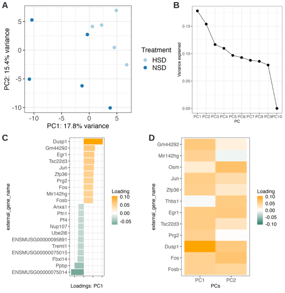
However, we can observe no separation of the groups along PC1 but rather by a combination of PC1 and PC2 (separation by a diagonal from middle top to bottom right) - hence high loadings on both principal components need to be assessed. For this, we switch to the ‘PCA_Loadings_Matrix’ panel. To see something meaningful, we need to adjust the default parameters at the bottom. From the previous loadings plot, we can deduce that the general loading levels are rather small - therefore, we adjust the ‘absolute loading threshold to filter entities with low impact’ to 0.05. As we are interested in PC1 and PC2, we adjust the number of PCs to include them as well (Fig. D3 D). We can confirm by visual inspection that Dusp1 has the combined highest impact, followed by Fos and Osm. Fos in combination with Jun are components of the AP-1 transcription factor complex and have been reported to play a role in inflammaging4. Osm is a gene that has been known to have inflammatory and anti-inflammatory effects5.
Statistical Analysis:
Following single interesting genes - Single Gene Visualisations:
To statistically test the two genes identified by their high loadings on PC1 and their difference in expression between the treatments, we can go to the Single Gene Visualisations tab. Here, single tests are performed and no multiple testing correction is done, allowing for a quick lookup of genes of interest. Checking Dusp1, Fos, Osm, and Ppbp, we obtain significant (p<0.05) results for all but Osm, with Dusp1 and Fos being upregulated in HSD compared to NSD, while Ppbp is downregulated (Fig. D4A).
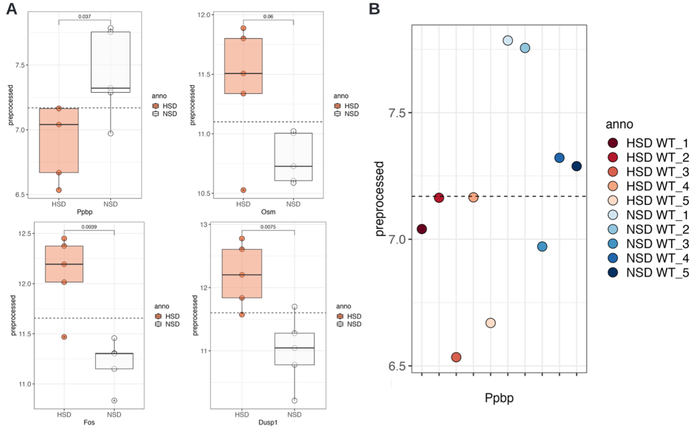
If we change the ‘groups to show the data for’ to ‘Simulation_Treatment’, we can observe for Ppbp that NSD_1 and NSD_2 and HSD_3 and HSD_5 behave differently from the other members of the group (Fig. D4B). This aligns with the PCA results. Note, that we cannot ‘test’ for a difference as we have a single data point for each.
Assessing all genes – Differential analysis:
We switch to the Differential analysis tab to analyse all genes at once. We want to compare the treatment groups, specifically HSD vs. NSD, taking the latter as control. The order is important to interpret the direction of up- and down-regulation but does not change anything in terms of significance. As we have chosen the DESeq2 pipeline, cOmicsArt automatically selects the appropriate test. We obtain 47 genes (0.29% of the entire set) with significant changes between the conditions. The majority (31 genes) are significantly upregulated (16 downregulated) with a chosen significance level of 0.05 (after Benjamini-Hochberg multiple testing correction) (Table D1).
The most significant gene is ENSMUSG00000044786 (ZFP36). To get an overview of actual effect sizes (fold changes), we subselect within the shown table to show only the significant genes by clicking into the respective padj column in the table (where ‘all’ stands). Here we can adjust the sliding bar to select only genes with a padj value in the determined range. A quick check at the bottom of the table confirms we only selected the 49 entries. We then sort the log2Fold changes by clicking on the little grey up and down arrows. The Log2Fold change range goes from -0.34 to 1.23. Switching to the visual representation of the table, we go to the tab Volcano. Setting a Log FC threshold of 0.5, we can see that 10 genes remain as significant highlights (Fig. D5).
| Gene | baseMean | log2FoldChange | pvalue | padj |
|---|---|---|---|---|
| ENSMUSG00000024190 | 3425.50 | 1.23 | 2.69E-04 | 1.38E-02 |
| ENSMUSG00000038418 | 3400.16 | 1.06 | 1.21E-05 | 1.18E-03 |
| ENSMUSG00000021250 | 3324.20 | 0.95 | 3.25E-06 | 5.20E-04 |
| ENSMUSG00000052684 | 875.64 | 0.76 | 3.56E-05 | 2.34E-03 |
| ENSMUSG00000031431 | 1159.30 | 0.72 | 2.37E-04 | 1.32E-02 |
| ENSMUSG00000044786 | 8404.73 | 0.71 | 2.37E-19 | 2.65E-16 |
| ENSMUSG00000052837 | 8531.19 | 0.60 | 1.24E-07 | 2.48E-05 |
| ENSMUSG00000020423 | 1718.03 | 0.58 | 1.33E-07 | 2.48E-05 |
| ENSMUSG00000053560 | 1702.31 | 0.56 | 1.55E-08 | 5.78E-06 |
| ENSMUSG00000021123 | 655.70 | 0.52 | 8.26E-06 | 9.99E-04 |
| ENSMUSG00000042265 | 990.08 | 0.48 | 2.49E-05 | 1.99E-03 |
| ENSMUSG00000055148 | 1430.02 | 0.47 | 1.15E-07 | 2.48E-05 |
| ENSMUSG00000071076 | 1220.37 | 0.46 | 3.42E-10 | 1.92E-07 |
| ENSMUSG00000026034 | 1026.68 | 0.44 | 2.39E-05 | 1.99E-03 |
| ENSMUSG00000059657 | 599.05 | 0.43 | 6.41E-05 | 3.77E-03 |
| ENSMUSG00000021134 | 1140.64 | 0.41 | 2.96E-05 | 2.20E-03 |
| ENSMUSG00000030142 | 775.57 | 0.35 | 5.19E-04 | 2.15E-02 |
| ENSMUSG00000035569 | 2044.15 | 0.32 | 1.26E-05 | 1.18E-03 |
| ENSMUSG00000026987 | 2535.04 | 0.30 | 8.92E-06 | 9.99E-04 |
| ENSMUSG00000047888 | 1138.43 | 0.29 | 1.87E-03 | 4.56E-02 |
| ENSMUSG00000021025 | 5177.26 | 0.29 | 1.21E-03 | 3.56E-02 |
| ENSMUSG00000031229 | 1653.37 | 0.29 | 4.03E-06 | 5.63E-04 |
| ENSMUSG00000040054 | 749.37 | 0.29 | 5.97E-04 | 2.30E-02 |
| ENSMUSG00000041235 | 738.21 | 0.28 | 5.51E-04 | 2.20E-02 |
| ENSMUSG00000058318 | 823.56 | 0.26 | 1.71E-03 | 4.44E-02 |
| ENSMUSG00000022521 | 915.62 | 0.25 | 1.60E-03 | 4.26E-02 |
| ENSMUSG00000000078 | 4568.06 | 0.24 | 7.86E-04 | 2.66E-02 |
| ENSMUSG00000030083 | 1691.89 | 0.23 | 1.79E-03 | 4.44E-02 |
| ENSMUSG00000008348 | 8243.71 | 0.23 | 4.03E-04 | 1.81E-02 |
| ENSMUSG00000042406 | 2495.90 | 0.21 | 7.13E-04 | 2.57E-02 |
| ENSMUSG00000034994 | 2752.88 | 0.19 | 7.66E-04 | 2.66E-02 |
| ENSMUSG00000020846 | 4210.24 | -0.17 | 3.91E-04 | 1.81E-02 |
| ENSMUSG00000059182 | 2211.07 | -0.18 | 1.32E-03 | 3.68E-02 |
| ENSMUSG00000022584 | 1659.75 | -0.18 | 5.07E-04 | 2.15E-02 |
| ENSMUSG00000028249 | 2915.46 | -0.21 | 1.39E-03 | 3.79E-02 |
| ENSMUSG00000040659 | 1452.83 | -0.21 | 1.09E-03 | 3.29E-02 |
| ENSMUSG00000022372 | 1751.24 | -0.21 | 2.06E-03 | 4.89E-02 |
| ENSMUSG00000069516 | 41354.07 | -0.21 | 3.96E-04 | 1.81E-02 |
| ENSMUSG00000020849 | 1157.78 | -0.23 | 6.29E-04 | 2.35E-02 |
| ENSMUSG00000059108 | 2624.48 | -0.23 | 1.24E-03 | 3.57E-02 |
| ENSMUSG00000021537 | 773.58 | -0.24 | 8.65E-04 | 2.77E-02 |
| ENSMUSG00000024142 | 782.36 | -0.24 | 8.14E-04 | 2.68E-02 |
| ENSMUSG00000064246 | 585.36 | -0.26 | 9.44E-04 | 2.93E-02 |
| ENSMUSG00000033213 | 3082.27 | -0.26 | 4.47E-05 | 2.78E-03 |
| ENSMUSG00000029322 | 1406.33 | -0.27 | 2.72E-04 | 1.38E-02 |
| ENSMUSG00000019960 | 1965.95 | -0.30 | 1.77E-03 | 4.44E-02 |
| ENSMUSG00000102051 | 1772.11 | -0.34 | 3.15E-05 | 2.20E-03 |
Table D1 Statistical analysis. Overview showing all significant genes from the comparison HSD vs NSD (adjusted p value < 0.05 and sorted by log2FoldChange(LFC)). Omitting the columns ‘lfcSE’, baseMean and ‘stat’.
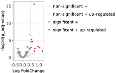
The set includes: ENSMUSG00000044786 (Zfp36), ENSMUSG00000052684 (Jun), ENSMUSG00000053560 (Ier2), ENSMUSG00000020423 (Btg2), ENSMUSG00000052837 (JunB), ENSMUSG00000021250 (Fos), ENSMUSG00000038418 (Egr1), ENSMUSG00000021123 (Rdh12), ENSMUSG00000031431 (TSC22D3), ENSMUSG00000024190 (Dusp1). Half of these genes have been associated with major functions of neutrophils, such as Egr1 for microbial killing, chemoattractant priming, NETosis, Fos, Btg2, and Dusp2 for small pore migration, and JunB for NETosis6. Further, Jun, Ier2, JunB, Fos, and Egr1 belong to the early immediate response, while Zfp36, TSC22D3 and Dusp1 belong to the glucocorticoid targets. We can conclude that besides no great global shifts, neutrophil core functions seem to be altered by High salt diet.
Set analysis - Heatmap & Enrichment Analysis:
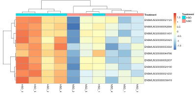
To obtain a nice visual representation, we switch to the heatmap panel and select for the row-selection Select based on Annotation - which means that we can select data based on their row annotation hence for example precisely their ID. We select the 10 genes which we just identified to be significantly upregulated. The resulting heatmap, after row-wise scaling, shows a distinct separation of the treatments, whereby the sample NSD_5 clusters close to HSD_1, which itself clusters away from the other HSD samples (Fig. D6).
We save the set of genes by clicking Save genes shown in Heatmap for OA within Enrichment Analysis tab’ to further use them for overrepresantation analysis. To further characterise the set we can perform an enrichment analysis. We switch to the Enrichment Analysis tab and select the gene set we just identified. As we have a set of genes we first perform an Over-representation analysis uploading the identified set of genes. We choose the set to test as KEGG, HALLMARK and GO_BP (biological process). As universe, we used all genes present after pre-processing. We obtain enriched terms for Hallmark such as TNFa signaling via NFkB, Hypoxia, UV response up, and P53 pathway (Fig. D7).
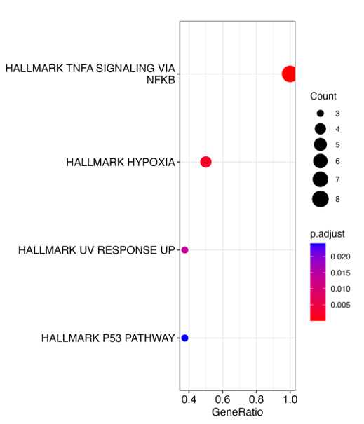
In addition to the visualisations we obtain the enrichment results as tables, telling us which query genes are within the respective (enriched) set. We can, for example, see, that 8 of our input genes belong to the term TNFa signalling via NFkB (Table D2).
| Description | GeneRatio | BgRatio | pvalue | p.adjust | geneID | Count |
|---|---|---|---|---|---|---|
| TNFA_SIGNALING_VIA_NFKB | 8/8 | 179/3573 | 3.41E-11 | 5.46E-10 | 12227/14281/19252/13653/22695/16476/16477/15936 | 8 |
| HYPOXIA | 4/8 | 163/3573 | 2.53E-04 | 2.03E-03 | 14281/19252/22695/16476 | 4 |
| UV_RESPONSE_UP | 3/8 | 135/3573 | 2.57E-03 | 1.37E-02 | 12227/14281/16477 | 3 |
| P53_PATHWAY | 3/8 | 182/3573 | 6.02E-03 | 2.41E-02 | 12227/14281/16476 | 3 |
| APOPTOSIS | 2/8 | 139/3573 | 3.61E-02 | 1.04E-01 | 12227/16476 | 2 |
| ESTROGEN_RESPONSE_LATE | 2/8 | 145/3573 | 3.90E-02 | 1.04E-01 | 14281/22695 | 2 |
Table D2 Enriched Hallmark terms. Only sets with at least two genes from the initial query set are shown.
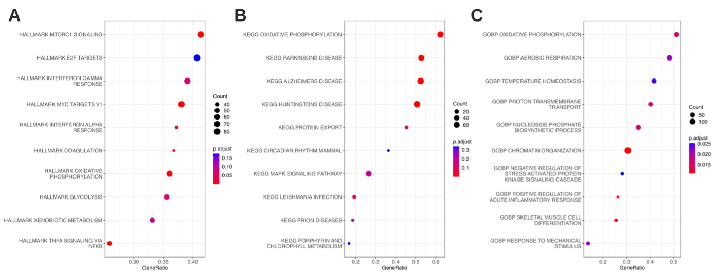
Overall we observed rather subtle differences, for which it can be challenging to determine a set of interest that requires setting a threshold, e.g. LFC. To avoid setting such an arbitrary threshold we performed a gene set enrichment analysis, which takes ranked entities into account, here chosen to be ranked by Log fold change (LFC). This approach is able to identify shifts of changes and is helpful if, for example, a single gene’s change is not deemed significant or with a large effect size. The visualization of the enriched hallmark terms reveals the terms MTORC1 signaling, Myc targets and Interferon alpha response, as well as Oxidative Phosphorylation. The latter is also obtained for the KEGG set, next to Alzheimer’s, Huntington’s, and Parkinson’s disease. GO also identified Oxidative Phosphorylation as an enriched term, along with chromatin organisation, temperature homeostasis, positive regulation of acute inflammatory response, and others (Fig. D8).
Considering the cell type (bone-marrow neutrophils), the studied cells seem to differ in their utilization of oxidative phosphorylation, which is a sign of differentiation for neutrophils7. Note that in the original publication[\^0], the ranking for GSEA was done based on t-test statistic values as well and a different DE-analysis was conducted as a basis; here it was done based on LFC values.
Intermediate summary
We saw that on a global scale, we could not observe a clear pattern to distinguish between the treatments. This is, for example, globally visible when assessing sample correlation, as the correlation is overall at a high level. When looking at the PCA, we can see a rather high spread of samples belonging to NSD, whereas the HSD samples are less spread within the dimension reduction plot. Additionally, the statistical analysis returns only a small set of differentially expressed genes, indicating that the treatment effect affects a smaller portion of the entire data set. When performing an overrepresentation analysis of the DE-genes, we obtain a clear signal for TNFa signaling via NFkB. When performing gene set enrichment analysis on the LFC-ranked genes among the most enriched terms oxidative phosphorylation stands out. This together suggests that the effect of the HSD treatment alters the cellular metabolism in a directed fashion to an inflammatory state.
For further analysis, one might be interested in subselecting the data to focus on the potentially relevant aspects. For this, one can add the information from the statistical analysis to the gene annotation. This information is within the results table and can be obtained from the differential analysis tab. Moreover, one could add information to the entities indicating whether they are associated with the term Oxidative phosphorylation (using GO as a resource) to be able to visualize that specific subset within the heatmap panel. Additionally, while it may not be appropriate in this context, one could consider adding information to the samples, such as marking potential outliers and then redoing the analysis.
Final Documentation
All of the figures shown here were also sent to the report during the analysis of the dataset. The full HTML report, including the figures, can be found in Supplementary E. Some notes were added to showcase how the report can replace additional notes and be self-sufficient. If you explore the report, you can also find some publication-ready snippets to incorporate into your methods section. Please note that while we’ve taken extensive measures to prevent data loss in the event of an unexpected crash of the web app, we cannot fully guarantee that it won’t occur. To safeguard your work, we recommend periodically saving your report. The analysis using cOmicsArt involved data retrieval, preparation, upload, and pre-processing, followed by a detailed investigation of sample correlation, PCA, and gene set enrichment to understand the subtle effects of HSD treatment in neutrophils.
References
-
Jeon, J. H., Hong, C. W., Kim, E. Y. & Lee, J. M. Current understanding on the metabolism of neutrophils. Immune Network vol. 20 1–13 Preprint at https://doi.org/10.4110/in.2020.20.e46 (2020) ↩
-
Tan, Y. et al. Dual specificity phosphatase 1 attenuates inflammation-induced cardiomyopathy by improving mitophagy and mitochondrial metabolism. Mol Metab 64, (2022) ↩
-
Piccardoni, P. et al. Thrombin-activated human platelets release two NAP-2 variants that stimulate polymorphonuclear leukocytes. Thromb Haemost 76, 780–785 (1996) ↩
-
Karakaslar, E. O. et al. Transcriptional activation of Jun and Fos members of the AP-1 complex is a conserved signature of immune aging that contributes to inflammaging. Aging Cell 22, e13792 (2023) ↩
-
Lantieri, F. & Bachetti, T. OSM/OSMR and Interleukin 6 Family Cytokines in Physiological and Pathological Condition. International Journal of Molecular Sciences 2022, Vol. 23, Page 11096 23, 11096 (2022) ↩
-
Jeon, J. H., Hong, C. W., Kim, E. Y. & Lee, J. M. Current understanding on the metabolism of neutrophils. Immune Network vol. 20 1–13 Preprint at https://doi.org/10.4110/in.2020.20.e46 (2020) ↩
-
Jeon, J. H., Hong, C. W., Kim, E. Y. & Lee, J. M. Current understanding on the metabolism of neutrophils. Immune Network vol. 20 1–13 Preprint at https://doi.org/10.4110/in.2020.20.e46 (2020) ↩