Moving from cOmicsArt to R: Customizing result visualisations and performing additional analyses

This showcase demonstrates how to use cOmicsArt to customize visualizations to fit, e.g., a publication style. Additionally, the obtained analysis script is adjusted to highlight the option of customizing the analysis itself.

For context, the metabolomics dataset used in this showcase comes from a study investigating the effect of maternal obesity on the liver health state of the offspring¹. The focus of the study is on Kupffer cells, liver-specific macrophages essential for liver development and functions. The findings reveal that maternal obesity disrupts Kupffer cell development in the fetus, leading to fatty liver disease and liver inflammation in the offspring. Among other data, serum metabolomics was obtained under different conditions, precisely variations in the diet — high fat diet (HFD) or control diet (CD) — of the mother, of the foster mother, i.e. the lactating female, and of the offspring. Therefore a condition termed for example ‘HFD CD CD’ specifies that the mother received HFD and the lactating female as well as the offspring CD. Serum metabolomics measurements were obtained from the offspring. When the mother receives an HFD, this is referred to as maternal obese otherwise as maternal lean.

The showcase is divided into three sections: ‘Data Upload and Pre-processing’, ‘PCA Analysis’ and ‘Additional Analysis’. The first section covers the transition from raw data to cOmicsArt and then to R, including basic customization. The second and third sections focus entirely on the analysis within R.

The Data Upload and Pre-processing

The data was received from Metabolon and prepared as detailed in the manuscript76. The obtained data sheets within an Excel workbook can be accessed from this repository (https://github.com/LeaSeep/MaternalObesity/tree/main/data – Metabolon.xlsx).

For uploading to cOmicsArt, the already pre-processed data matrix was transposed to fit the format accepted by cOmicsArt and then saved as a CSV file. Information about the metabolites, such as the pathways they belong to and additional identifiers, was placed in a separate row annotation table. Similarly, details about the samples were collected and organized into an independent sample annotation matrix for cOmicsArt. The original ‘CHEM_IDs’ were numerical, which could be mistaken with indexes when used as row names. To resolve this, the prefix ‘CHEM_ID’ was added to all IDs within the data matrix and the row annotation table. Additionally, the hyphens (‘-‘) within the sample names were replaced with underscores (‘_’), as hyphens are not allowed as column names inside cOmicsArt.

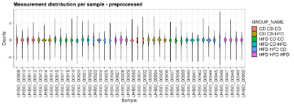
The three data matrices were uploaded to cOmicsArt with no data selection performed. Also ‘None’ was chosen as pre-processing, due to the data pre-processing done outside the app. From the diagnostic plots colored after ‘GROUP_NAME’ we can observe that each distribution is centered around zero and a wide distribution of ranges between the samples. Due to the amount of samples, the plot is compressed. To obtain a decompressed plot one can receive the R code and data by pressing on the respective button. Upon executing the obtained script within RStudio, the violin plots are immediately obtained and shown in the plots viewer panel of RStudio. Within RStudio’s export functionality, one can adjust the plotting area manually to enlarge the plot area and hence decompress the plot (Fig E1).

Figure E1: Metabolomics measurement distribution per sample. The plot is manually adjusted within Rstudio’s plot panel to enlarge the plotting area and decompress the visualisation.

PCA Analysis

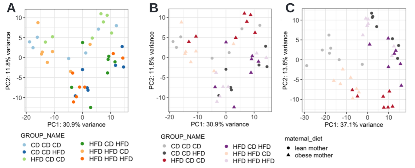
A PCA analysis is conducted to identify differences in the global metabolome between the maternal obese group and the maternal lean group. When the data is colored by ‘GROUP_NAME’, it becomes evident that the offspring’s diet (hence the last diet out of the triplet) is the major contributing factor (Fig E2A). However, with the six groups displayed, distinguishing them is not straightforward. While one could define new groups, such as maternal lean v.s. maternal obese or offspring on CD v.s. HFD, to simplify the coloring, it is more useful to keep the groups separate and use similar colors to indicate similarities besides differing groups. This customization is not possible within the cOmicsArt user interface. However, users can obtain the R code and data to replicate the entire analysis, from data input to PCA visualization.

Figure E2: PCA visualisation and analysis customisation. A The original cOmicsArt generated PCA plot on batch-corrected data with default coloring. B Customised PCA-plot on the basis of obtained R script and data from cOmicsArt. The shape of the dots now resembles the maternal dietary status while the color theme was adjusted. C Customised batch correction, now supplying a model matrix, leads to a different appearing PCA result, leading still to the same conclusion.

The provided script allows for instant and self-sufficient reproducibility. By executing the script, the same PCA plot is obtained as a ggplot25 object, which provides the basis for customisation. Here, an additional shape argument is given to indicate the mother’s diet (CD vs HFD) and the color scheme was updated (Fig. E2B). Since ggplot is widely used, large language models like ChatGPT or GitHub Copilot can reliably assist in adjusting the code to meet specific needs. One might note that we have not yet recreated the exact plot shown in the manuscript. The reason is that the two analyses differ in their batch correction procedure. When supplying a model matrix to the combat function, which biases the batch correction to retain as much variance as possible, which can be attributed to the variable of interest — in this case, ‘GROUP_NAME’, we could recreate the exact plot (Fig E2C) from the original publication. After these adjustments, the plot underscores that the most significant variance in the metabolomic data is due to the offspring’s diet, rather than the mother’s diet.

Additional analysis

The straightforward approach to replicate cOmicsArt’s results allow also for easy expansion of the analysis, through the reuse of code snippets or building upon supplied data in a convenient data object. We demonstrate how the PCA script can be reused for a different dataset. Then, the resulting PCA model is used to project left-out samples onto the constructed PCA space. Finally, we utilize the computed and projected principal components to quantify how predictive the offspring diet is within a machine-learning-based approach. Note that the complete code snippet – obtained from cOmicsArt and then expanded as described in the following – can be found in Supplementary.

The provided PCA code snippet can be re-used to compute and display a PCA with a different dataset. Here, we perform a PCA with a subset of mice, precisely those that were born to mothers on CD, subsequently lactated by a foster mother on CD and received HFD and CD, respectively. The subsetted data object can either be used to overwrite the original data for direct reuse of the snippet or the code snippet needs to be adjusted to work with the new object.

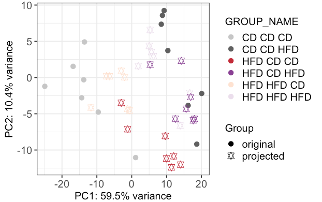
The obtained PCA was then used to transform the left-out samples (i.e., those with differing maternal diets) to project them into the new PCA space. This approach allows us to visually assess how well the offspring’s diet alone can separate samples with varying maternal diets. To avoid confusion, we added a ‘p’ to the group names of the projected samples. By adjusting the ‘GROUP_NAME’ column instead of adding a new column, we could simply re-use the previous plotting command. The resulting PCA (Fig. E3) shows that the offspring diet drives the separation, even the samples with differing maternal diets, indicating that the variance in the metabolome data is mainly attributed to the offspring’s diet.

Figure E3: Projection PCA. Basis of PCA is built upon samples belonging to the group CD CD CD or CD CD HFD, while all other samples are projected onto that space, indicating how sufficient the offspring’s diet is to separate the remaining samples according to their offspring diets regardless of their mother’s diet.

While one can visually confirm that the offspring diet is the major source of variance within the metabolome data, we haven’t quantified this. One possible quantification is by determining the predictive power of the offspring diet in predicting the offspring diet of the remaining samples with differing maternal diets. As descriptors for each sample, we use all the principal components from the above-described procedure (14 components). Due to the small sample size, we use k-nearest neighbors (k-NN) as the machine learning model, which does not require training but only the specification of the parameter k (the number of neighbors to consider), which is set to 3. Upon implementation, a prediction accuracy of 82% indicates a good prediction performance based solely on the offspring’s diet. Assessing the true and false positive rates reveals a significant difference (0.6 vs. 0). The difference indicates that some samples with a true offspring CD are misclassified as having an offspring HFD (Table E1A). Further analysis of the respective maternal diets shows that the misclassified samples are from maternal obese, combined with an offspring diet of CD (Table E1B). Interestingly, this is not observed with an offspring diet of HFD. These findings highlight that while the offspring diet is the primary source of differences in the metabolome, the maternal diet, in combination with a CD offspring diet, induces detectable changes in the metabolome, making it more similar to that of an HFD offspring.

A		Actual			B	Actual
		CD	HFD			HFD	CD	CD	HFD
Predicted	CD	7	0	Predicted	CD	2	0	5	0
	HFD	7	14		HFD	5	7	2	7

Table E1 Confusion matrices of kNN-based offspring-diet prediction. A Confusion matrix indicating the correct classification of all HFD offspring samples, whereby seven additional actual CD samples have been wrongly predicted as HFD samples. B Confusion matrix showing the actual complete condition (of mothers and offspring) highlights that only samples with obese mothers on offspring kept on CD are misclassified as offspring on HFD.

The ability to access and customize code snippets directly from cOmicsArt significantly enhances the flexibility and depth of analysis for researchers. By providing the underlying R code, cOmicsArt not only allows for easy replication of visualizations and results but also allows users to extend and tailor their analyses to their needs and questions.

References

1. Mass, E. et al. Developmental programming of Kupffer cells by maternal obesity causes fatty liver disease in the offspring. (2023) doi:10.21203/RS.3.RS-3242837/V1. ↩